
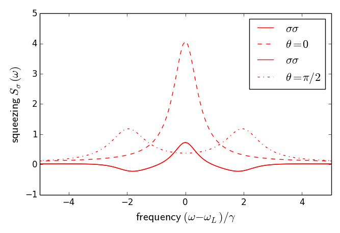
Squeezing correlations (left) and spectra (right) for a two-level atom. Parameters as in the script.
#!/usr/bin/python
# -*- coding: utf-8 -*-
"""
Resonance fluorescence with the regression formula (SS 2017, QO II).
We have a routine that solves the Bloch equations with initial data
pe, pg, sigma (dipole). If one applies the regression hypothesis, we
need an initial state \sigma \rho whose expectation values are
Tr[ \pi_e \sigma \rho ] = 0,  since \sigma = |g>,
Tr[ \sigma \sigma \rho ] = 0,
Tr[ \sigma^\dag \sigma \rho ] = <\pi_e>
* Note that complex conjugation does not hold any longer!
* This means that we have to re-write the equations in such a way
  that conjugation is not 'hard-wired'.
"""

from pylab import *
from scipy.integrate import odeint

xsize = 6.5
ysize = 1.1*xsize*0.5*(sqrt(5.) - 1.)
mysize = 16

def setParameters(theta0 = 1.0*pi, phi0 = 0.):
    # theta0 = pi (0) is ground (excited) state
    """
    set parameters for two-level dynamics (Bloch equations)
    cw = True: cw laser
    cw = False: pulsed laser (length pulse_tau)
    c0 = initial condition for two-level vector (pure state)
    t = vector of times 0 < t < tMax where solution is plotted
    (default) initial conditions with optional parameters theta0, phi0
    """
    global Rabi_f, Laser_f, Atom_f, Gamma_eg, gamma_e, cw, pulse_tau, c0, t, N_t, dt, \
           Omega, Rabi_env

    gamma_e = 1.
    Gamma_eg = (0.0 + 0.5)*gamma_e # minimum value is 0.5*gamma_e
    Atom_f = 200.*gamma_e
    Laser_f = Atom_f + 0.0*gamma_e
    Rabi_f = 2.0*gamma_e*exp(+0.0*pi*1j)
    cw = True # False = pulsed laser
    # pulse area is Rabi_f * sqrt(2*pi) * pulse_tau
    pulse_tau = pi/abs(Rabi_f)/sqrt(2*pi)
#    pulse_tau = 0.075/gamma_e
#    pulse_tau = 1./gamma_e
    if cw:
        def Omega(t):
            return 2.*real(Rabi_f*exp(-1j*Laser_f*t))
        def Rabi_env(t):
            return Rabi_f*ones_like(t)
    else:
        def Omega(t):
            return 2.*real(Rabi_f*exp(-1j*Laser_f*t))*exp(-0.5*((t - pulse_tau)/pulse_tau)**2)
        def Rabi_env(t):
            return Rabi_f*exp(-0.5*((t - pulse_tau)/pulse_tau)**2)

    # initial conditions, parametrized by angle theta0 on Bloch sphere,
    # theta0 = 0 is excited state ('spin up')
    # phi0 is relative phase, fixes phase of initial dipole
    #
    cg0, ce0 = sin(0.5*theta0)*exp(-1j*0.5*phi0), cos(0.5*theta0)*exp(1j*0.5*phi0)
    c0 = (cg0, ce0)
    # important to signal that c0 has complex entries, otherwise
    # the conversion to real pairs does not work
    c0 = array(c0, dtype=complex)

    # interesting time interval
    tMax = 3./gamma_e
    tMax = 24.*max(3./gamma_e, 3.*pi/(gamma_e + abs(Rabi_f)))
    N_t = 1024
    t, dt = linspace(-0.0*pulse_tau, tMax, N_t, retstep = True)

    return

def steady_state(trace_0 = 1.):
    global Rabi_f, Laser_f, Atom_f, Gamma_eg, gamma_e

    Delta_L = Laser_f - Atom_f
    denom = 0.5*gamma_e + 0.5*abs(Rabi_f)**2*Gamma_eg/(Gamma_eg**2 + Delta_L**2)
    inversion = -0.5*gamma_e / denom
    dipole = 0.5j*Rabi_f*inversion/(Gamma_eg - 1j*Delta_L)
    pe = 0.5*(trace_0 + inversion)
    pg = 0.5*(trace_0 - inversion)
    return [pg, pe, dipole]

def BlochL_rwa(state, t):
    """
    Bloch equations ('superoperator or Liouvillian L')
    worked out for complex observables with the RWA
    'state' = [pg, pe, sigma], this is *not* the Bloch vector!
    """
    global Rabi_f, Laser_f, Atom_f, Gamma_eg, gamma_e
    (pg, pe, sigma) = state
    dotsigma = -1j*(Atom_f - Laser_f)*sigma - Gamma_eg*sigma + \
               0.5*1j*Rabi_env(t)*(pe - pg)
    dotpe = - gamma_e*pe - imag(conj(Rabi_env(t))*sigma)
    dotpg = - dotpe
    return [dotpg, dotpe, dotsigma]


def r_BlochL_rwa(x, t, *args):
# mapping of BlochL to function of real parameters
    state = x.view(complex128)
    dstatedt = BlochL_rwa(state, t, *args)
    return asarray(dstatedt, dtype=complex128).view(float64)


def xBlochL_rwa(xstate, t):
    """
    extended Bloch equations ('superoperator or Liouvillian L')
    not assuming that  = conj()
    'xstate' = [pg, pe, sigma, sigmaDag]
    """
    global Rabi_f, Laser_f, Atom_f, Gamma_eg, gamma_e
    (pg, pe, sigma, sigmaDag) = xstate
    dotsigma = -1j*(Atom_f - Laser_f)*sigma - Gamma_eg*sigma + \
               0.5*1j*Rabi_env(t)*(pe - pg)
    dotsigmaDag = 1j*(Atom_f - Laser_f)*sigmaDag - Gamma_eg*sigmaDag - \
               0.5*1j*conj(Rabi_env(t))*(pe - pg)
    dotpe = - gamma_e*pe + 0.5j*(conj(Rabi_env(t))*sigma - Rabi_env(t)*sigmaDag)
    dotpg = - dotpe
    return [dotpg, dotpe, dotsigma, dotsigmaDag]

def r_xBlochL_rwa(x, t, *args):
# mapping of xBlochL to function of real parameters
    state = x.view(complex128)
    dstatedt = xBlochL_rwa(state, t, *args)
    return asarray(dstatedt, dtype=complex128).view(float64)


if False:
    # solve equations of motion, compare two versions of Bloch equations
    #
    setParameters()
    print('solve two-level equations')

    # solve with dissipation the Bloch equations, using the
    # same initial state
    (cg0, ce0) = c0
    state0 = [abs(cg0)**2, abs(ce0)**2, conj(cg0)*ce0]
    # 'extended state', with complex conjugate (sigmaDag) separately
    xstate0 = [abs(cg0)**2, abs(ce0)**2, conj(cg0)*ce0, cg0*conj(ce0)]
    #
    # again, need to specify that these are tuples of complex numbers
    state0 = array(state0, dtype=complex)
    xstate0 = array(xstate0, dtype=complex)

    # solve the Bloch equations (RWA version only)
    #
    rwa = odeint(r_BlochL_rwa, state0.view(float64), t, full_output = 1)
    rwa = rwa[0].view(complex128)
    #
    bg_rwa = real(rwa[:,0])
    be_rwa = real(rwa[:,1])
    sigma_rwa = rwa[:,2]

    xrwa = odeint(r_xBlochL_rwa, xstate0.view(float64), t, full_output = 1)
    xrwa = xrwa[0].view(complex128)
    #
    bg_xrwa = real(xrwa[:,0])
    be_xrwa = real(xrwa[:,1])
    sigma_xrwa = xrwa[:,2]
    sigmaDag_xrwa = xrwa[:,3]

    # analytical solution for steady state
    #
    [pg, pe, dipole] = steady_state()

if True:
    #
    setParameters()
    print('solve two-level correlations')

    # analytical solution for steady state
    #
    [pg, pe, dipole] = steady_state()

    # solve Bloch equations in the regression sense, take
    # modified initial state from sigma rho_ss and from sigma rho_ss sigmaDag
    # (intensity correlations)
    #
    xstate_ss = [dipole, 0., 0., pe]
    xstate_ss = array(xstate_ss, dtype=complex)

    # solve the RWA version of Bloch equations
    #
    corr = odeint(r_xBlochL_rwa, xstate_ss.view(float64), t, full_output = 1)
    corr = corr[0].view(complex128)
    #
    bg_corr = real(corr[:,0])
    be_corr = real(corr[:,1])
    sigma_corr = corr[:,2]
    sigmaDag_corr = corr[:,3]

    # for intensity correlations
    xstate_ss = [pe, 0., 0., 0.] # should be the ground state
    xstate_ss = array(xstate_ss, dtype=complex)

    g2 = odeint(r_xBlochL_rwa, xstate_ss.view(float64), t, full_output = 1)
    g2 = g2[0].view(complex128)
    #
    bg_g2 = real(g2[:,0])
    be_g2 = real(g2[:,1]) # this is the G2(tau) correlation function
    sigma_g2 = g2[:,2]
    sigmaDag_g2 = g2[:,3]

    # for squeezing correlations, quadrature phase
    theta = 0.5*pi
    xstate_ss = [exp(1j*theta)*dipole, exp(-1j*theta)*conj(dipole), \
                 exp(-1j*theta)*pg, exp(1j*theta)*pe]
    xstate_ss = array(xstate_ss, dtype=complex)

    sq_corr = odeint(r_xBlochL_rwa, xstate_ss.view(float64), t, full_output = 1)
    sq_corr = sq_corr[0].view(complex128)
    #
    sq_sigma = sq_corr[:,2]
    sq_sigmaDag = sq_corr[:,3]
    sq_theta = exp(1j*theta)*sq_sigma + exp(-1j*theta)*sq_sigmaDag

if False:
    # extract final (stationary?) state, can be compared to
    # analytical results
    #
    g_ss = bg_rwa[-1]
    e_ss = be_rwa[-1]
    sigma_ss = sigma_rwa[-1]

    g_xss = bg_xrwa[-1]
    e_xss = be_xrwa[-1]
    sigma_xss = sigma_xrwa[-1]
    sigmaDag_xss = sigmaDag_xrwa[-1]

    print('stationary state (standard / complexified)')
    print('at time %3.4g / gamma_e' %(gamma_e*t[-1]))
    print('p_e = %3.4g (%3.4g)' %(e_ss, e_xss))
    print('p_g = %3.4g (%3.4g)' %(g_ss, g_xss))
    print('p_e + p_g = %3.4g (%3.4g)' %(e_ss + g_ss, e_xss + g_xss))

    print('sigma = %3.4g + %3.4g i (%3.4g + %3.4g i, %3.4g + %3.4g i)'
           %(real(sigma_ss), imag(sigma_ss), real(sigma_xss), imag(sigma_xss),
                                     real(sigmaDag_xss), -imag(sigmaDag_xss)))

    print('theory:')
    print('p_e = %3.4g' %(pe))
    print('p_g = %3.4g' %(pg))

    print('sigma = %3.4g + %3.4g i' %(real(dipole), imag(dipole)))

if False:
   figure(2, (xsize, ysize), tight_layout = True)
   plot( t, bg_rwa, 'b', lw = 1.5, label = 'g' )
   plot( t, be_rwa, 'r', lw = 1.5, label = 'e' )
   plot( t, real(sigma_rwa), 'g', lw = 1.5, label = '$\mathsf{Re\ }d$' )
   plot( t, imag(sigma_rwa), 'g--', lw = 1.5, label = '$\mathsf{Im\ }d$' )

if False:
   figure(2, (xsize, ysize), tight_layout = True)
   plot( t, bg_xrwa, 'b+', label = 'g' )
   plot( t, be_xrwa, 'r+', label = 'e' )
   plot( t, real(sigma_xrwa), 'g+', label = '$\mathsf{Re\ }d$' )
   plot( t, imag(sigma_xrwa), 'g+', label = '$\mathsf{Im\ }d$' )
   plot( t, real(sigmaDag_xrwa), '.' )
   plot( t, -imag(sigmaDag_xrwa), '.' )
   ylim(-1, 1)
   legend()

if False:
    """
    compute spectrum of dipole correlation function,
    should return Mollow triplet
    """

    ddcorr = sigmaDag_corr - sigmaDag_corr[-1]
    print('check stationary value of C_sigma: %3.4g + %3.4g i vs %3.4g'
           %(real(sigmaDag_corr[-1]), imag(sigmaDag_corr[-1]), abs(dipole)**2) )
    spec = 2*real(dt*fft(ddcorr))

    figure(4, (xsize, ysize), tight_layout = True)
    plot( t, real(sigmaDag_corr), 'b' )
    plot( t, imag(sigmaDag_corr), 'r' )

    t_max = 12./gamma_e
    xlim(0, t_max)
    plot( [0, t_max], [abs(dipole)**2, abs(dipole)**2], ':' )

    spec = fftshift(spec)
    omega = fftshift(2*pi*fftfreq(N_t, d = dt))

    figure('Mollow', (xsize, ysize), tight_layout = True)
    plot(omega/gamma_e, spec, 'r-')
    om_max = max(2.5*sqrt(abs(Rabi_f)**2 + (Laser_f - Atom_f)**2), 3.*gamma_e)

    xlim(-om_max, om_max)
    xlabel(r'$\mathsf{frequency\ } (\omega - \omega_L)/\gamma$', size = mysize)
    ylabel(r'$\mathsf{spectrum\ } S_d( \omega )$', size = mysize)


if True:
    """
    compute 'squeezing spectrum' of correlation Q_sigma(t) =
    """

    sqcorr = sigma_corr
    print('check stationary value of Q_sigma: %3.4g + %3.4g i vs %3.4g + %5.4g i'
           %(real(sqcorr[-1]), imag(sqcorr[-1]), \
             real(dipole**2), imag(dipole**2)) )

    # make plot of correlation function
    figure(4, (xsize, ysize), tight_layout = True)
    plot( t, real(sqcorr), 'b', label = 'Re Q' )
    plot( t, imag(sqcorr), 'r', label = 'Im Q' )


    # repeat for sigma_theta correlation function
    sTheta_corr = sq_theta
    dipole_theta = exp(1j*theta)*dipole + exp(-1j*theta)*conj(dipole)
    print('check stationary value of C_theta: %3.4g + %3.4g i vs %3.4g + %5.4g i'
           %(real(sTheta_corr[-1]), imag(sTheta_corr[-1]), \
             real(dipole_theta**2), imag(dipole_theta**2)) )

    plot( t, real(sTheta_corr), 'b--', label = r'$\mathsf{Re\ }C_\theta$' )
    plot( t, imag(sTheta_corr), 'r--', label = r'$\mathsf{Im\ } C_\theta$' )

    t_max = 12./gamma_e
    xlim(0, t_max)
    plot( [0, t_max], [real(dipole**2), real(dipole**2)], 'g:' )
    plot( [0, t_max], [imag(dipole**2), imag(dipole**2)], 'g:' )

    plot( [0, t_max], [real(dipole_theta**2), real(dipole_theta**2)], 'g:' )
    plot( [0, t_max], [imag(dipole_theta**2), imag(dipole_theta**2)], 'g:' )

    xlabel(r'$\mathsf{time\ } \gamma t$', size = mysize)
    ylabel(r'$\mathsf{correlation\ } Q_\sigma( t )$', size = mysize)
    legend(fontsize = mysize, loc = 'upper right')

    # subtract asymptotic value and take Fourier transform
    sqcorr -= sqcorr[-1]
    spec = 2*real(dt*fft(sqcorr)) # not obvious that this is the right rule
    # since the 'squeezing spectrum' can in general be complex
    #
    spec = fftshift(spec)
    omega = fftshift(2*pi*fftfreq(N_t, d = dt))

    figure('squeezing', (xsize, ysize), tight_layout = True)
    plot(omega/gamma_e, spec, 'r-', label = r'$\sigma\sigma$')

    # repeat for squeezing correlation
    #
    sTheta_corr -= sTheta_corr[-1]
    spec = 2*real(dt*fft(sTheta_corr)) # standard rule
    # because \sigma_\theta is hermitean
    #
    spec = fftshift(spec)
    plot(omega/gamma_e, spec, 'r--', label = r'$\sigma_\theta\sigma_\theta$')

    om_max = max(2.5*sqrt(abs(Rabi_f)**2 + (Laser_f - Atom_f)**2), 3.*gamma_e)
    xlim(-om_max, om_max)
    xlabel(r'$\mathsf{frequency\ } (\omega - \omega_L)/\gamma$', size = mysize)
    ylabel(r'$\mathsf{squeezing\ } S_\sigma( \omega )$', size = mysize)
    legend(fontsize = mysize)

if False:
    """
    compute spectrum by Fourier transform of excited state pe(t),
    gives intensity correlations
    """
    # plot correlation function
    figure(2, (xsize, ysize), tight_layout = True)
    plot( gamma_e*t, be_rwa, 'r' )
    plot( gamma_e*t, be_xrwa, 'b' )

    plot( gamma_e*t, be_g2/pe, 'k', lw = 1.5 )

    t_max = 5./gamma_e
    xlim(0, t_max)
    ylim(0, 1.05*max(be_rwa))
    plot( [0, t_max], [pe, pe], ':', c = 'gray' )
    xlabel(r'$\mathsf{time\ delay\ } \gamma_e \tau$', size = mysize)
    ylabel(r'$\mathsf{correlation\ } C_I(\tau)$', size = mysize)

    IIcorr = be_rwa - be_rwa[-1] # subtract final value
    spec = 2*real(dt*fft(IIcorr))

    IIcorr = be_xrwa - be_xrwa[-1]
    xspec = 2*real(dt*fft(IIcorr))

    # plot spectrum
    figure(1, (xsize, ysize), tight_layout = True)

    spec = fftshift(spec)
    xspec = fftshift(xspec)
    omega = fftshift(2*pi*fftfreq(N_t, d = dt))

    plot(omega/gamma_e, spec, 'r-')
    plot(omega/gamma_e, xspec, 'b-')
    om_max = max(6*abs(Rabi_f), 8*gamma_e)

    xlim(-om_max, om_max)
    xlabel(r'$\mathsf{frequency\ } (\omega - \omega_L)/\gamma$', size = mysize)
    ylabel(r'$\mathsf{spectrum\ } S_I( \omega )$', size = mysize)


show(block = False)
Squeezing correlations (left) and spectra (right) for a
two-level atom. Parameters as in the script.