#!/usr/bin/python
# -*- coding: utf-8 -*-
"""
solve Bloch-Lorenz equations for single-mode laser,
coupled to two-level medium.
"""

from pylab import *
from scipy.integrate import odeint

global pumpRate, gammaI, gammaP, kappa, deltaC, delta

Q_plot = True
xsize = 9.5
ysize = xsize*0.5*(sqrt(5.) - 1.)
mysize = 20; tsize = mysize - 4

def BlochLorenz(y, t):
    """
    Bloch-Lorenz three-variable Bloch-Lorenz equations
    Variables are [F, P, inv] with
    F = field (complex amplitude), damping kappa, detuning deltaC
    P = polarization (complex), damping gammaP, detuning delta
    inv = inversion (real), damping 2 gammaI, pumping pumpRate
    """
    global pumpRate, gammaI, gammaP, kappa, deltaC, delta

    # restore components of variable vector
    F = y[0];
    P = y[1];
    inv = y[2];

    # simplest semiclassical laser model with medium and cavity
    # dynamics, must be re-interpreted as real function for 
    # Python ODE integrator (see r_BlochLorentz below)
    #
    Fdot = -(kappa + 1j*deltaC)*F + 1j*kappa*P;
    Pdot = -(gammaP + 1j*delta)*P - 1j*gammaI*(F*inv);
    invDot = -2*gammaI*inv + pumpRate + gammaI*imag(conj(F)*P);

    # steady state solutions
    # F = 1j*kappa*P/(kappa + 1j*deltaC);
    # P = -i*gammaP*(F*inv)/(gammaP + 1j*delta);
    # inv = (pumpRate + gammaI*imag(conj(F)*P))/(2*gammaI);

    # collect output variables in vector
    return [ Fdot, Pdot, invDot ]

def r_BlochLorenz(x, t, *args):
# map defined on real parameters
    y = x.view(complex128)
    dydt = BlochLorenz(y, t, *args)
    return asarray(dydt, dtype=complex128).view(float64)

def steadyState(t_end, dt_end = 0.1, Q_error = False):
    """
    analyze steady state
    """
    global pumpRate, gammaI, gammaP, kappa, deltaC, delta
    # initial data
    #
    F_0 = 0.3*1j # field amplitude, need some small "seeding value"
    P_0 = 0.0*1j # polarisation
    inv_0 = 0. # inversion, a negative value could also be used, but
    # its magnitude would be somewhat arbitrary
    #
    # parameters
    #
    gammaI, gammaP = 1., 10.
    kappa = 1.0*gammaP
    deltaC = -1.1*kappa # laser (cavity, field) detuning
    delta = 1.1*kappa # medium polarisation detuning
    f_shift = 1. # common frequency shift does not affect intensities
    delta += f_shift
    deltaC += f_shift

    # time interval
    nb_t = 100
    t = linspace(0., t_end, nb_t)
        # convert complex initial data to real
    y_0 = array([F_0, P_0, inv_0], dtype = complex)
    outode = odeint(r_BlochLorenz, y_0.view(float64), t, args = (), full_output = 1)
    outode = outode[0].view(complex128)
    #
    F_t = outode[:,0]
    P_t = outode[:,1]
    inv_t = real(outode[:,2])
    # imInv_t = imag(outode[:,2]) # checked that imaginary part is zero as it should

    # 'measure' stationary values from last 10% of time 
    t_meas = (1. - dt_end)*t_end #
    i_meas = find(t >= t_meas)
    I_stat = mean(abs(F_t[i_meas])**2)
    dI_stat = std(abs(F_t[i_meas])**2)
    P2_stat = mean(abs(P_t[i_meas])**2)
    dP2_stat = std(abs(P_t[i_meas])**2)
    inv_stat = mean(inv_t[i_meas])
    dInv_stat = std(inv_t[i_meas])

    if Q_error:
        print('relative errors in stationary states')
        print('dI / I = %4.4g' %(dI_stat/I_stat))
        print('dP^2 / P^2 = %4.4g' %(dP2_stat/P2_stat))
        print('d inv / inv = %4.4g' %(dInv_stat/inv_stat))
    
    return I_stat, P2_stat, inv_stat


if True:
    # initial data
    F_0 = 0.3*1j # field amplitude
    P_0 = 0.01*1j # polarisation
    P_0 = 0.0*1j # polarisation
    inv_0 = 0. # inversion

    # parameters
    #
    gammaI, gammaP = 1., 2.
    pumpRate = 5.2*gammaI
    kappa = 2.0*gammaP
    deltaC = -0.1*kappa # laser (cavity, field) detuning
    delta = 0.1*kappa # medium polarisation detuning
    f_shift = 0.1*kappa # common frequency shift does not affect intensities
    delta += f_shift
    deltaC += f_shift

    # time interval
    nb_t = 300
    t_end = 30./gammaI
    t = linspace(0., t_end, nb_t)

    # --- differential equation solver ---
    # odeint evaluates the solution immediately (no object syntax required)
    # convert complex initial data to real
    y_0 = array([F_0, P_0, inv_0], dtype = complex)
    outode = odeint(r_BlochLorenz, y_0.view(float64), t, args = (), full_output = 1)
    outode = outode[0].view(complex128)
    #
    F_t = outode[:,0]
    P_t = outode[:,1]
    inv_t = real(outode[:,2])
    # imInv_t = imag(outode[:,2]) # checked that imaginary part is zero as it should

    # 'measure' stationary values from last 10% of time 
    t_meas = 0.9*t_end #
    i_meas = find(t >= t_meas)
    I_stat = mean(abs(F_t[i_meas])**2)
    dI_stat = std(abs(F_t[i_meas])**2)
    P2_stat = mean(abs(P_t[i_meas])**2)
    dP2_stat = std(abs(P_t[i_meas])**2)
    inv_stat = mean(inv_t[i_meas])
    dInv_stat = std(inv_t[i_meas])
    print('Bloch-Lorenz model solved to time gamma_I t = %3.3g ' %(gammaI*t_end))
    print('stationary data')
    print('   field intensity %4.4g +- %4.4g' %(I_stat, dI_stat))
    print("   polar'n intensity %4.4g +- %4.4g" %(P2_stat, dP2_stat))
    print('   inversion %4.4g +- %4.4g' %(inv_stat, dInv_stat))

    if Q_plot:
        figure(1, figsize = (xsize, ysize), tight_layout = True)
        plot( gammaI*t, inv_t, label = 'inversion' )
        plot( gammaI*t, abs(F_t)**2, lw = 2, label = 'intensity' )
        plot( gammaI*t, abs(P_t)**2, '--', label = '|pol|^2' )
        xlabel( r'$\mathsf{time\ } \gamma_I t$', size = mysize)
        legend(loc = 'upper right', fontsize = mysize)
        xticks(size = tsize); yticks(size = tsize)

Q_pumpScan = False

if Q_pumpScan:
    # scan pump rate and make a plot of laser threshold
    nb_p = 15
    pump_s = linspace(0.2*pumpRate, 1.5*pumpRate, nb_p)
    I_s = zeros(nb_p)
    inv_s = zeros(nb_p)
    for ii, pumpRate in enumerate(pump_s):
        print ii,
        I_stat, P2_stat, inv_stat = steadyState(t_end, Q_error = True)
        I_s[ii] = I_stat
        inv_s[ii] = inv_stat
    #
    figure(2, figsize = (xsize, ysize), tight_layout = True)
    plot( pump_s / gammaI, I_s, label = 'intensity' )
    plot( pump_s / gammaI, inv_s, label = 'inversion' )
    xlabel( r'$\mathsf{pump\ rate\ } R / \gamma_I$', size = mysize)
    legend(loc = 'upper left', fontsize = mysize)
    xticks(size = tsize); yticks(size = tsize)



show(block=False)

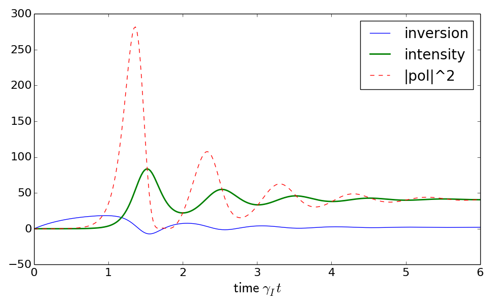
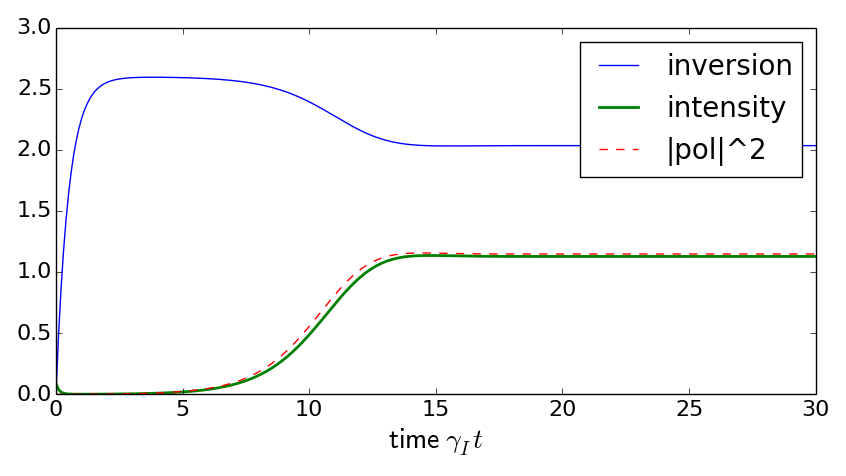
Solutions of the Lorentz model: intensity of the cavity mode, inversion of the medium, modulus squared of the medium polarisation. Arbitrary units, time in units of the decay time for the inversion. (left) large pumping rate (right) smaller pumping rate, just above threshold. For even smaller rates, the intensity stays zero at all times. Initial values: medium in ground state, cavity field with small amplitude. For large pumping, one observes relaxation oscillations before the system settles into a stationary state.