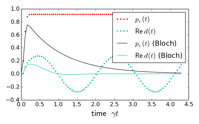
Excitation of a two-level-system with a short pulse: results of the Schrödinger equation (dotted) and the Bloch equations (solid).
#!/usr/bin/python
# -*- coding: utf-8 -*-
"""
Quantum Optics I, C. Henkel, WS 17/18
solve Bloch equations for a two-level system,
without the resonance approximation (also known as
'rotating wave approximation' RWA)
complex Rabi frequency Omega(t), also pulsed (envelope),
pictures in the Bloch sphere (not shown in lecture).
Note: change 'if True:' into 'if False:' to skip certain plots.
"""

from pylab import *
from scipy.integrate import odeint

# (re)define some standard size for plots and fonts
#
mysize = 16
tsize = 18
xsize = 6.5
ysize = xsize*0.5*(sqrt(5)-1)
plt.rcParams['figure.figsize'] = (xsize, ysize)
plt.rcParams['figure.autolayout'] = True
plt.rcParams['font.size'] = tsize-4
plt.rcParams['axes.labelsize'] = tsize+2
plt.rcParams['xtick.labelsize'] = tsize-4
plt.rcParams['ytick.labelsize'] = tsize-4

# set parameters and initial data
#
def setParameters(theta0 = 0.0*pi, phi0 = 0., Q_print = False):
    theta0 = pi # pi (0) is ground (excited) state
    """
    set parameters for two-level dynamics (Bloch equations)
    cw = True: cw laser
    cw = False: pulsed laser (length pulse_tau)
    c0 = initial condition for two-level vector (pure state)
    t = vector of times 0 < t < tMax where solution is plotted
    (default) initial conditions with optional parameters theta0, phi0
    """
    global Rabi_f, Laser_f, Atom_f, Gamma_eg, gamma_e, cw, pulse_tau, c0, t, dt, \
           Omega, Rabi_env

    gamma_e = 1.
    Gamma_eg = (2.0 + 0.5)*gamma_e # minimum value is 0.5*gamma_e
    Atom_f = 200.*gamma_e
    Atom_f = 200.*gamma_e
    Detuning =  - 3.*gamma_e
    Laser_f = Atom_f + Detuning
    Rabi_f = -20.0*gamma_e*exp(+0.*pi*1j)
    pulsed = True # True = pulsed laser
    # pulse area is Rabi_f * sqrt(2*pi) * pulse_tau
    pulse_tau = pi/abs(Rabi_f)/sqrt(2*pi)
#    pulse_tau = 0.075/gamma_e
#    pulse_tau = 1./gamma_e
    if not(pulsed):
        def Omega(t):
            return 2.*real(Rabi_f*exp(-1j*Laser_f*t))
        def Rabi_env(t):
            return Rabi_f*ones_like(t)
    else:
        def Omega(t):
            return 2.*real(Rabi_f*exp(-1j*Laser_f*t))*exp(-0.5*((t - pulse_tau)/pulse_tau)**2)
        def Rabi_env(t):
            return Rabi_f*exp(-0.5*((t - pulse_tau)/pulse_tau)**2)

    # initial conditions, parametrized by angle theta0 on Bloch sphere,
    # theta0 = 0 is excited state ('spin up' or 'North pole')
    # phi0 is relative phase, fixes phase of initial dipole
    #
    cg0, ce0 = sin(0.5*theta0)*exp(-1j*0.5*phi0), cos(0.5*theta0)*exp(1j*0.5*phi0)
    c0 = (cg0, ce0)

    # interesting time interval
    Nb_t = 40
    tMax = 3./gamma_e
    Nb_t = 80
    tMax = 4.3/gamma_e
    tMax = max(tMax, 3.*pi/(gamma_e + abs(Rabi_f)))
    t, dt = linspace(-0.0*pulse_tau, tMax, Nb_t, retstep = True)

    if Q_print:
        print('|Rabi| = %3.4g gamma' %(abs(Rabi_f)/gamma_e))
        if pulsed:
            print('laser pulse ~ %3.4g/gamma' %(pulse_tau*gamma_e))
        else:
            print('cw laser')
        print '(c_e(0), c_g(0)) = ',; print(c0[1::-1])
        print('time 0 (%3.4g) ... %3.4g / gamma' %(gamma_e*dt, gamma_e*tMax))
    return


def RabiH(c, t):
    global Rabi_f, Laser_f, Atom_f, Gamma_eg, gamma_e
    """
    two-level Hamiltonian applied to vector of amplitudes c = [g(t), e(t)]
    written in rotating frame at laser frequency, but not making RWA

    i d ce / d t = 0.5*Omega(t)*exp(1j*Laser_f*t)*cg - 0.5*(Laser_f - Atom_f)*ce
    i d cg / d t = 0.5*Omega(t)*exp(-1j*Laser_f*t)*ce + 0.5*(Laser_f - Atom_f)*cg

    """
    (cg, ce) = c
    dotce = -1j*(0.5*Omega(t)*exp(1j*Laser_f*t)*cg - 0.5*(Laser_f - Atom_f)*ce)
    dotcg = -1j*(0.5*Omega(t)*exp(-1j*Laser_f*t)*ce + 0.5*(Laser_f - Atom_f)*cg)
    return [dotcg, dotce]

def RabiH_rwa(c, t):
    global Rabi_f, Laser_f, Atom_f, Gamma_eg, gamma_e
    """
    two-level Hamiltonian in resonance approximation (rotating wave, RWA),
    in same rotating frame as RabiH, but fast rotating terms dropped

    i d ce / d t = 0.5*Rabi_f*cg - 0.5*(Laser_f - Atom_f)*ce
    i d cg / d t = 0.5*conj(Rabi_f)*ce + 0.5*(Laser_f - Atom_f)*cg

    """
    (cg, ce) = c
    dotce = -1j*(0.5*Rabi_env(t)*cg - 0.5*(Laser_f - Atom_f)*ce)
    dotcg = -1j*(0.5*conj(Rabi_env(t))*ce + 0.5*(Laser_f - Atom_f)*cg)
    return [dotcg, dotce]


"""
The differential equation is solved with the command
odeint(r_Rabi, c0.view(float64), t, full_output = 1)
r_Rabi: command that provides the time derivative, working
        with real input and output
c0: initial condition, pair of complex numbers
t: times where the solution is computed (a vector)

Challenge: 'odeint' works with real-valued functions.
The translation from complex to real numbers is done
in Python with the 'view' command. A complex number z
can be converted into a pair of real numbers (with some
floating point precision) with x = z.view(float64).
The reverse is done with z = x.view(complex128).

The following code transforms the function RabiH that
works with complex numbers c = (cg, ce) into a function
that accepts real numbers. Code inspired from
http://stackoverflow.com/questions/19910189/
scipy-odeint-with-complex-initial-values#19921629
"""
def r_Rabi(x, t, *args):
    c = x.view(complex128)
    dcdt = RabiH(c, t, *args)
    return asarray(dcdt, dtype=complex128).view(float64)

def r_Rabi_rwa(x, t, *args):
    c = x.view(complex128)
    dcdt = RabiH_rwa(c, t, *args)
    return asarray(dcdt, dtype=complex128).view(float64)

def BlochL(state, t):
    """
    Bloch equations ('superoperator or Liouvillian L')
    worked out for complex observables
    'state' = [pg, pe, sigma], this is *not* the Bloch vector!
    This does *not* work for correlation functions (regression
    theorem) where some symmetries of the density operator are
    no longer present.
    """
    global Rabi_f, Laser_f, Atom_f, Gamma_eg, gamma_e
    (pg, pe, sigma) = state
    dotsigma = -1j*(Atom_f - Laser_f)*sigma - Gamma_eg*sigma + \
               0.5*1j*Omega(t)*exp(1j*Laser_f*t)*(pe - pg)
    dotpe = - gamma_e*pe - \
               imag(Omega(t)*sigma*exp(-1j*Laser_f*t))
    dotpg = - dotpe
    return [dotpg, dotpe, dotsigma]

def BlochL_rwa(state, t):
    """
    Bloch equations ('superoperator or Liouvillian L')
    worked out for complex observables with the RWA
    'state' = [pg, pe, sigma], this is *not* the Bloch vector!
    Same limitation as BlochL for regression calculations,
    restricted to 'one-time observables'.
    """
    global Rabi_f, Laser_f, Atom_f, Gamma_eg, gamma_e
    (pg, pe, sigma) = state
    dotsigma = -1j*(Atom_f - Laser_f)*sigma - Gamma_eg*sigma + \
               0.5*1j*Rabi_env(t)*(pe - pg)
    dotpe = - gamma_e*pe - imag(conj(Rabi_env(t))*sigma)
    dotpg = - dotpe
    return [dotpg, dotpe, dotsigma]

def r_BlochL(x, t, *args):
# mapping of BlochL to function of real parameters
    state = x.view(complex128)
    dstatedt = BlochL(state, t, *args)
    return asarray(dstatedt, dtype=complex128).view(float64)

def r_BlochL_rwa(x, t, *args):
# mapping of BlochL to function of real parameters
    state = x.view(complex128)
    dstatedt = BlochL_rwa(state, t, *args)
    return asarray(dstatedt, dtype=complex128).view(float64)

if True:
    # solve equations of motion, pure-state case with Rabi Hamiltonian first
    #
    print('solve two-level equations')
    setParameters(Q_print = True)

    # important to signal that c0 has complex entries, otherwise
    # the conversion to real pairs does not work
    c0 = array(c0, dtype=complex)
    sol = odeint(r_Rabi, c0.view(float64), t, full_output = 1)
    sol = sol[0].view(complex128)
    #
    # extract the probability amplitudes from the solution
    cg = sol[:,0]
    ce = sol[:,1]

    # now, solve the same problem with the resonance approximation (RWA)
    #
    rwa = odeint(r_Rabi_rwa, c0.view(float64), t, full_output = 1)
    rwa = rwa[0].view(complex128)
    #
    # extract the probability amplitudes from the solution
    cg_rwa = rwa[:,0]
    ce_rwa = rwa[:,1]

    # take meaningful quantities
    pe_t = abs(ce)**2
    pg_t = abs(cg)**2
    dipole_t = conj(cg)*ce
    P = pe_t + pg_t

    # take meaningful quantities
    pe_rwa = abs(ce_rwa)**2
    pg_rwa = abs(cg_rwa)**2

    # now include dissipation (spontaneous decay, dephasing) and
    # solve the Bloch equations, using the same initial state
    (cg0, ce0) = c0
    state0 = [abs(cg0)**2, abs(ce0)**2, conj(cg0)*ce0]
    #
    # again, need to specify that this is a tuple of complex numbers
    state0 = array(state0, dtype=complex)
    sol = odeint(r_BlochL, state0.view(float64), t, full_output = 1)
    sol = sol[0].view(complex128)
    #
    bg_t = real(sol[:,0])
    be_t = real(sol[:,1])
    sigma_t = sol[:,2]

    # repeat with RWA version of Bloch equations
    #
    rwa = odeint(r_BlochL_rwa, state0.view(float64), t, full_output = 1)
    rwa = rwa[0].view(complex128)
    #
    bg_rwa = real(rwa[:,0])
    be_rwa = real(rwa[:,1])
    sigma_rwa = rwa[:,2]

if True:
    # test whether numerical solution has real-valued populations
    # switch to 'if False:' if this block is no longer of interest
    fg = figure('0 reality test')
    plot( gamma_e*t, imag(sol[:,0]), 'b', label = r'$\mathsf{Im\ }p_g$' )
    plot( gamma_e*t, imag(sol[:,1]), 'r', label = r'$\mathsf{Im\ }p_e$' )

    plot( gamma_e*t, imag(rwa[:,0]), 'b+', label = r'$\mathsf{Im\ }p_g$, rwa' )
    plot( gamma_e*t, imag(rwa[:,1]), 'r+', label = r'$\mathsf{Im\ }p_e$, rwa' )

    xlabel( r'time $\gamma_e t$')
    ylabel( r'imag part of populations')
    legend()
    fg.set_tight_layout(True)

if True:
    # check norm of Bloch vector (= 1 for pure states)
    fg = figure('1 norm of Bloch vector')

    # Hamiltonian case, should be = 1
    norm_H = sqrt((pe_t - pg_t)**2 + 4*abs(dipole_t)**2)
    plot( gamma_e*t, norm_H, 'k', label = r'$\mathsf{Schr\"odinger}$' )

    # norm of Bloch vector (related to purity of state)
    norm_B = sqrt((be_t - bg_t)**2 + 4*abs(sigma_t)**2)
    plot( gamma_e*t, norm_B, 'b', label = r'$\mathsf{Bloch eqn}$' )

    norm_rwa = sqrt((be_rwa - bg_rwa)**2 + 4*abs(sigma_rwa)**2)
    plot( gamma_e*t, norm_rwa, 'b+', label = r'$\mathsf{Bloch + rwa}$' )

    # add also sum of probabilities, should be = 1 at all times
    #
    plot( gamma_e*t, P, 'k.', label = '$\mathsf{total\ } p(t)$, Schr.' )
    plot( gamma_e*t, be_t + bg_t, 'b.', label = '$\mathsf{total\ } p(t)$, Bloch' )

    xlabel( r'time $\gamma_e t$')
    ylabel( r'norm $|{\bf s}(t)|$')
    legend()
    fg.set_tight_layout(True)


# compare Hamiltonian and Bloch models
#
if True:
    fh = figure('2 Schroedinger vs Bloch')
    # plot data from Hamiltonian dynamics
    plot( gamma_e*t, pe_t, 'k.--', label = '$p_e(t)$' )
    plot( gamma_e*t, pg_t, 'k.--', label = '$p_g(t)$' )
    #
    # add data from Bloch equations (incl damping)
    plot( gamma_e*t, be_t, 'b-', label = '$p_e(t)$ (Bloch)' )
    plot( gamma_e*t, bg_t, 'm-', label = '$p_g(t)$ (Bloch)' )

    legend(loc = 'upper right')
    xlabel(r'$\mathsf{time\ }\, \gamma t$')
    ylabel('$\mathsf{populations}$')
    fh.set_tight_layout(True)


# compare Hamiltonian and Bloch models
#
if True:
    fh = figure('3 Schroedinger vs Bloch: dipole')
    # plot data from Hamiltonian dynamics
    plot( gamma_e*t, pe_t, 'r.', label = '$p_e(t)$' )
    #    plot( gamma_e*t, pg_t, 'b', label = '$p_g(t)$' )
    plot( gamma_e*t, real(conj(cg)*ce), 'c.', label = '$\mathsf{Re\ } d(t)$' )
    #
    # add data from Bloch equations (incl damping)
    plot( gamma_e*t, be_t, 'k-', label = '$p_e(t)$ (Bloch)' )
    plot( gamma_e*t, real(sigma_t), 'c-', label = '$\mathsf{Re\ } d(t)$ (Bloch)' )

    legend(loc = 'upper right')
    xlabel(r'$\mathsf{time\ }\, \gamma t$')
    fh.set_tight_layout(True)


# illustrate RWA for Hamiltonian model
#
if True:
    fh = figure('4 Hamiltonian: test RWA')
    # plot data from Hamiltonian dynamics
    plot( gamma_e*t, pe_t, 'r.', label = '$p_e(t)$' )
    plot( gamma_e*t, pe_rwa, 'r-', label = '$p_e(t)$, rwa' )
    #    plot( gamma_e*t, pg_t, 'b', label = '$p_g(t)$' )
    #    plot( gamma_e*t, P, 'k', label = '$\mathsf{total\ } p(t)$' )
    plot( gamma_e*t, real(conj(cg)*ce), 'c.', label = '$\mathsf{Re\ } d(t)$' )
    plot( gamma_e*t, real(conj(cg_rwa)*ce_rwa), 'c-', label = '$\mathsf{Re\ } d(t)$, rwa' )

    legend(loc = 'upper right')
    xlabel(r'$\mathsf{time\ }\, \gamma t$')
    fh.set_tight_layout(True)

# illustrate RWA for Bloch model
#
if True:
    fh = figure('5 Bloch: test RWA')
    #
    # data from Bloch equations (incl damping)
    plot( gamma_e*t, be_t, 'k', label = '$p_e(t)$ (Bloch)' )
    plot( gamma_e*t, real(sigma_t), 'c', label = '$\mathsf{Re\ } d(t)$ (Bloch)' )

    plot( gamma_e*t, be_rwa, 'k.', label = '$p_e(t)$ (Bloch), rwa' )
    plot( gamma_e*t, real(sigma_rwa), 'c.', label = '$\mathsf{Re\ } d(t)$ (Bloch), rwa' )

    legend(loc = 'center right')
    xlabel(r'$\mathsf{time\ }\, \gamma t$')
    fh.set_tight_layout(True)


# illustrate absorption and stimulated emission

if False:
    fh = figure('absorption, stimulated emission')
    #
    # data from Bloch equations (incl damping)
    # dipole is sigma_rwa, plot imaginary part, defined by
    # projection onto (negative) complex Rabi frequency

    plot( gamma_e*t, - imag(conj(Rabi_env(t))*sigma_rwa)/abs(Rabi_f), 'g', \
          label = '$\mathsf{Im\ } d(t) \mathsf{\ (abs/em)}$' )

    plot( gamma_e*t, - real(conj(Rabi_env(t))*sigma_rwa)/abs(Rabi_f), 'c--', \
          label = '$\mathsf{Re\ } d(t)$' )

    plot( gamma_e*t, be_rwa, 'k', lw = 2., label = '$\mathsf{excited\ } p_e(t)$' )

    plot( gamma_e*t, -real(Rabi_env(t))/abs(Rabi_f), 'r', label = '$\mathsf{Re\ } E(t)/|\mathsf{max\,} E|$' )

    legend(loc = 'upper right')
    xlabel(r'$\mathsf{time\ }\, \gamma t$')
    fh.set_tight_layout(True)


# plot entropy and purity vs time
#
if False:
    fh = figure(5)

    # norm_B = sqrt((be_t - bg_t)**2 + 4*abs(sigma_t)**2)
    # print('end: norm(B) = %4.4g' %(norm_B[-1]))
    # purity = 0.5*(1. + norm_B**2)
    # ent = - 0.5*(1. + norm_B)*log(0.5*(1. + norm_B))
    # for ii, nrm in enumerate(norm_B):
    #     if nrm < 1:
    #         ent[ii] -= 0.5*(1. - nrm)*log(0.5*(1. - nrm))
    #
    # plot( t, purity, 'm.-', label = 'purity' )
    # plot( t, ent, 'b.-', label = 'entropy' )

    norm_B = sqrt((be_rwa - bg_rwa)**2 + 4*abs(sigma_rwa)**2)
    print('end: norm(B) = %4.4g' %(norm_B[-1]))
    purity = 0.5*(1. + norm_B**2)
    ent = - 0.5*(1. + norm_B)*log(0.5*(1. + norm_B))
    for ii, nrm in enumerate(norm_B):
        if nrm < 1:
            ent[ii] -= 0.5*(1. - nrm)*log(0.5*(1. - nrm))

    plot( gamma_e*t, 0*0.59 + purity, 'm.', label = 'purity (RWA)' )
    plot( gamma_e*t, ent, 'b.', label = 'entropy (RWA)' )

    xlabel(r'$\mathsf{time\ } \gamma t$')
    legend(loc = 'center right')

# plot solutions in Bloch sphere, two projections
#
if False:
    fh = figure(4, (2*ysize, ysize))
    plot_s1 = False
    # make projection of 13 plane (or 23 plane)
    nscut = subplot(121)
    nscut.set_aspect(1)
    nscut.add_patch(Circle((0,0), radius = 1, color = 'lightgray', lw = 2))
    nscut.text(-0.9, 0.9, '$|\Omega| =\, %4.4g \,\gamma$' %(abs(Rabi_f)/gamma_e), fontsize = mysize)
    nscut.text(-0.9, 0.75, '$\Delta =\, %4.4g \,\gamma$' %((Laser_f - Atom_f)/gamma_e), fontsize = mysize)

    nscut.text(-0.08, 0.95, '$|e\\rangle$', fontsize = mysize)
    nscut.text(-0.08, -0.95, '$|g\\rangle$', fontsize = mysize)

    eqcut = subplot(122)
    eqcut.set_aspect(1)
    eqcut.add_patch(Circle((0,0), radius = 1, color = 'lightgray', lw = 2))

#
    s3 = be_rwa - bg_rwa
    s1, s2 = 2.*real(sigma_rwa), -2*imag(sigma_rwa)

    if plot_s1:
        nscut.plot( s1, s3, 'b.-' )
    else:
        nscut.plot( s2, s3, 'b.-' )
    eqcut.plot( s1, s2, 'm.-' )


    sca(nscut)
    xlim(-1.1, 1.1); ylim(-1.1, 1.1)
    if plot_s1:
        xlabel('1 = Re(d)'); ylabel('3')
    else:
        xlabel('2 = -Im(d)'); ylabel('3')
    sca(eqcut)
    xlim(-1.1, 1.1); ylim(-1.1, 1.1)
    xlabel('Re(d)'); ylabel('Im(d)')


# plot evolution of a 'swarm' of initial conditions
#
if False:

    phiT = [0., 0.125*pi, 0.25*pi, 0.375*pi, 0.5*pi]
    thetaT = [0.55*pi, 0.5*pi, 0.45*pi]

    fh = figure(6, (2*xsize, xsize))
    nscut = subplot(121)
    nscut.set_aspect(1)
    nscut.add_patch(Circle((0,0), radius = 1, color = 'lightgray', lw = 2))
    nscut.text(-0.9, 0.9, '$|\Omega| =\, %4.4g \,\gamma$' %(abs(Rabi_f)/gamma_e), fontsize = mysize)
    nscut.text(-0.9, 0.75, '$\Delta =\, %4.4g \,\gamma$' %((Laser_f - Atom_f)/gamma_e), fontsize = mysize)

    nscut.text(-0.08, 0.95, '$|e\\rangle$', fontsize = mysize)
    nscut.text(-0.08, -0.95, '$|g\\rangle$', fontsize = mysize)

    eqcut = subplot(122)
    eqcut.set_aspect(1)
    eqcut.add_patch(Circle((0,0), radius = 1, color = 'lightgray', lw = 2))


    for theta0 in thetaT:
        for phi0 in phiT:

            setParameters(theta0 = theta0, phi0 = phi0)
            # theta0 = pi (0) is ground (excited) state

            # now solve with dissipation and RWA the Bloch equations, using this
            # initial (pure) state
            (cg0, ce0) = c0
            state0 = [abs(cg0)**2, abs(ce0)**2, conj(cg0)*ce0]
            #
            # again, need to specify that this is a tuple of complex numbers
            state0 = array(state0, dtype=complex)
            rwa = odeint(r_BlochL_rwa, state0.view(float64), t, full_output = 1)
            rwa = rwa[0].view(complex128)
            #
            bg_rwa = real(rwa[:,0])
            be_rwa = real(rwa[:,1])
            sigma_rwa = rwa[:,2]

            s3 = be_rwa - bg_rwa
            s1, s2 = 2.*real(sigma_rwa), -2*imag(sigma_rwa)

            nscut.plot( s1, s3, '.-' )
            eqcut.plot( s1, s2, '.-' )

    sca(nscut)
    xlim(-1.1, 1.1); ylim(-1.1, 1.1)
    xlabel('1 = Re(d)'); ylabel('3')
    sca(eqcut)
    xlim(-1.1, 1.1); ylim(-1.1, 1.1)
    xlabel('Re(d)'); ylabel('Im(d)')


show(block=False)
Excitation of a two-level-system with a short pulse:
results of the Schrödinger equation (dotted) and the
Bloch equations (solid).