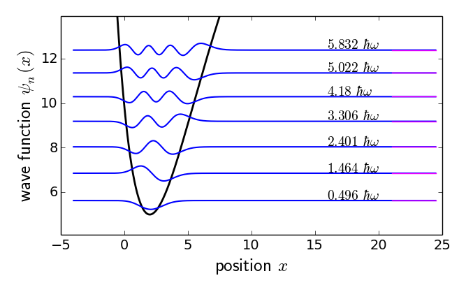
Low-energy spectrum of the Morse potential. Magenta lines on right: exact energy eigenvalues.
#!/usr/bin/python
#
"""
Solve Schroedinger equation in Morse potential using a
finite-difference scheme. This script / function assumes
as input parameters
x:  discrete position grid,
    assumed equidistant for the moment
D, a, r0, V0: Morse parameters
Et: target energy eigenvalue,
    sometimes we need eigenfunctions above the ground level,
    centered around a laser frequency, for example
"""

tsize = 18
xsize = 6.5
ysize = xsize*0.5*(sqrt(5)-1)
plt.rcParams['figure.figsize'] = (xsize, ysize)
plt.rcParams['figure.autolayout'] = True
plt.rcParams['font.size'] = tsize-2
plt.rcParams['axes.labelsize'] = tsize
plt.rcParams['xtick.labelsize'] = tsize-4
plt.rcParams['ytick.labelsize'] = tsize-4

from pylab import *
from scipy.sparse import diags
from scipy.sparse.linalg import eigsh
from scipy.sparse import csc_matrix

# convergence checks that are possible:
# -- is the grid large enough? (are the highest states still bound?)
# -- is the grid fine enough? (accuracy of eigenvalues)


if True:
    # the following relatively arbitrary parameters
    # are the default values
    nb_levels = 3;
    D = 20.; a = 5.; r0 = 2.; V0 = 5.; Et = 10.; # and grid x
    #
    nb_x = 256 + 128 + 128
    x0, x1 = r0 - 1.2*a, r0 + 4.5*a
    x_g, dx = linspace(x0, x1, nb_x, retstep = True)

    # order of the finite-difference scheme for the second derivative
    # = 2 (= 4 ) is a second (fourth) order scheme. Computation time is
    # roughly the same, but the fourth order scheme is superior in accuracy,
    # compared to exact solution.
#    stencil = 2
    stencil = 4

def solve_Morse(D = 20., a = 5., r0 = 2., V0 = 5., Et = 10., \
                nb_levels = 3, x = x_g, Q_plot = False):
    """
    Solve Schroedinger equation for the Morse potential
    D(1 - exp(-(z - r0)/a))**2 + V0
    levels, states = solve_Morse()
    levels: list (length nb_levels) with eigenvalues
    states: array (size(x), nb_levels) with wave functions

    Meaning of parameters:
    D: dissociation energy
    V0: minimum energy
    a: length parameter
    r0: equilibrium bond length
    Et: targeted energy eigenvalue
    nb_levels: number of eigenvalues
    x: spatial grid (must be equidistant)
    Q_plot = False: plot the solution

    The script makes a few simple checks whether the grid is
    wide enough. Boundary conditions assumed:
    Dirichlet on inner side
    Neumann on outer side
    Can be adjusted by changing in the script the definition
    of type_BC = ['D', 'N'] (inner, outer).
    """
    # type of boundary conditions at left and right end
    type_BC = ['D', 'N']
    # D: Dirichlet
    # N: Neumann
    #
    nb_x = shape(x)[0]
    x0, x1 = x[0], x[-1]
    dx = min(abs(diff(x)))
    if abs(dx - max(diff(x))) > 1e-5*dx:
        print('... non-equidistant grid: sorry to return nonsense')
    #
    def morse(z):
        return D*(1. - exp(-(z - r0)/a))**2 + V0
#        return D*((z - r0)/a)**2 + V0
#         return V0*ones(size(z))
    # make a few tests of grid size, turning points at target energy Et
    if Et < V0:
        print('Error: increase Et above V0 = %4.4g' %(V0))
    if (morse(x[0]) < Et) | (morse(x[-1]) < Et):
        print('Error: turning points not in grid')
    #
    # set up Schroedinger matrix
    #
    h = 0.5; # hbar^2 / (2 m) in front of second derivative
    hb_omega = sqrt(2.*h*2.0*D/a**2); # harmonic approximation
    x_e = hb_omega / (4.*D); # anharmonicity parameter
    # checked that the Morse spectrum is indeed
    # E_k = V0 + hb_omega*(k + 1/2) - hb_omega*x_e*(k + 1/2)**2
    #

    # try to understand convergence towards exact eigenvalues
    # it is indeed a question of step size! It seems that
    # with a smaller step (up to 1700 points were no problem numerically)
    # the agreement with the exact spectrum becomes better and better.
    # The width of the grid must be large enough, too, of course.
    #
    # Another idea: try to use a 'five-point stencil' for the second
    # derivative: accuracy improves from O(dx^2) to O(dx^4) -- works
    # very well, and I did not see any increase in computing time ...
    #
    # From https://en.wikipedia.org/wiki/Finite_difference_coefficient
    # replace band matrix with diagonals (1, -2, 1) [/dx**2]
    # by band matrix with entries (-1./12, 4./3, -2.5, 4./3, -1./12) [/dx**2]
    # guess that Dirichlet boundary condition is handled as before,
    # while Neumann BC (at the left end, e.g.) boils down to replacing
    # by the four-point stencil (., 5./4, -2.5, 4./3, -1./12 [/dx**2])
    # or by the three-point stencil (., ., -1.25, 4./3, -1./12 [/dx**2])
    #
    if stencil == 2: # (1, -2, 1) [/dx**2]
        diag_0 =  h*2./dx**2 + morse(x)
        diag_1 = -h*1./dx**2
        for b in [0,1]:
            if type_BC[b] == 'N':
                # adjust diagonal values at the end for Neumann b.condition
                diag_0[-b] = morse(x[-b]) + h*1./dx**2
        # sparse (banded) matrix from diagonals, secondary diags are -1 and +1
        Schroed = diags([diag_1, diag_0, diag_1], [-1, 0, 1], shape = (nb_x, nb_x))
    #
    elif stencil == 4: # (-1./12, 4./3, -2.5, 4./3, -1./12) [/dx**2]
        diag_0 =  h*2.5/dx**2 + morse(x)        # need the arrays
        diag_1 = -h*(4./3)/dx**2 * ones(nb_x-1) # here for the BC
        diag_2 =  h*(1./12)/dx**2
        for b in [0,1]:
            if type_BC[b] == 'N':
                # 1st line (., ., -1.25, 4./3, -1./12 [/dx**2])
                # 2nd line (., 5./4, -2.5, 4./3, -1./12 [/dx**2])
                # adjust diagonal (-1,0,1) values at the end for Neumann b.condition
                # (just a guess, not obvious!)
                diag_0[-b] = morse(x[-b]) + h*1.25/dx**2
                diag_1[-b] = -h*1.25/dx**2
        # sparse (banded) matrix from diagonals, secondary diags are -1 and +1
        Schroed = diags([diag_2, diag_1, diag_0, diag_1, diag_2], [-2,-1, 0, 1, 2], \
                        shape = (nb_x, nb_x))
    #
    #              eigsh is the (sparse) solver for symmetric/hermitean problems
    # transform to 'column-indexed sparse coordinates'
    Schroed = csc_matrix(Schroed)
    level, state = eigsh(Schroed, k = nb_levels, sigma = Et, \
                         mode = 'normal', which = 'LM')
    # sigma: find eigenvalues around Et
    # mode: related to re-scaling of eigenvalues
    # which: L(argest) M(agnitude) for 1/(E - Et)
    if Q_plot:
        # make plot of found wave functions
        scale_psi = 0.5/sqrt(dx)
        offset_E = 0.03*scale_psi
        L = x1 - x0
        mysize = 18; tsize = mysize - 4

        plot( x, morse(x), 'k', lw = 2. )
        for k in range(nb_levels):
            scaled_Ek = (level[k] - V0) / hb_omega # re-scaled to convenient unit
            plot( x, level[k] + scale_psi*state[:,k], 'b', linewidth = 1.5 )
#            plot( [x[0], x[-1]], [level[k], level[k]], c = 'gray', linewidth = 1.0 )
            text( x1 - 0.3*L, level[k] + offset_E, \
#                  '$E_{%i}\,=\,%4.4g\,\hbar\omega$' %(k, scaled_Ek), \
                  '$%4.4g\,\hbar\omega$' %(scaled_Ek), \
                  fontsize = tsize, clip_on=True)
        # add numbers for exact Morse eigenvalues
        for k in range(int(2*D/hb_omega)):
            expected_k = V0 + hb_omega*(k + 1./2) - hb_omega*x_e*(k + 1./2)**2
            if (expected_k - min(level) > -0.45*hb_omega) & \
               (expected_k - max(level) < 0.45*hb_omega):
                scaled_k = (expected_k - V0) / hb_omega
                plot( [x1 - 0.12*L, x1], [expected_k, expected_k], \
                      c = 'magenta', linewidth = 1.0 )
#                text( x1 - 0.12*L, expected_k + offset_E, '$%4.4g$' %(scaled_k), \
#                      fontsize = tsize, clip_on=True)

        xticks(size = tsize), yticks(size = tsize)
        ylim(min(level) - 1.2*hb_omega, max(level) + 1.2*hb_omega)
        xlabel( '$\mathsf{position}\, x$', fontsize = mysize )
        ylabel( '$\mathsf{wave\,functions}\, \psi_n(x)$', fontsize = mysize )
        show(block=False)

    return level, state

# show(block=False)
Low-energy spectrum of the Morse potential. Magenta lines on right:
exact energy eigenvalues.