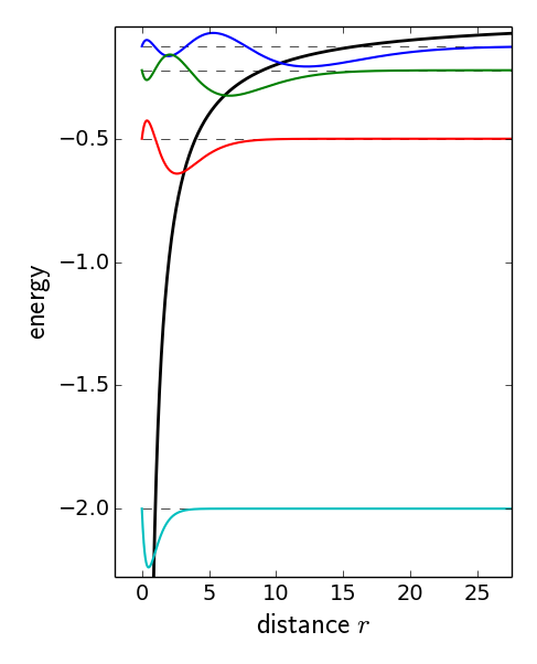
Hydrogen-like wave functions in the Coulomb potential of the Helium nucleus.
#!/usr/bin/python
# -*- coding: utf-8 -*-
"""
2019 Nov 15, C. Henkel
Play with Hartree-Fock theory for the Helium ground state.
"""

from pylab import *
from scipy.integrate import odeint, quad, trapz
from scipy.sparse import diags, coo_matrix, csc_matrix
from scipy.sparse.construct import eye
# sparse eigenvalue solver:
from scipy.sparse.linalg import eigs, eigsh, spsolve

# adapt a few parameters for size and font size of figures
# other global parameters are set in the configuration file
# matplotlibrc that is to be placed in the directory
# ~/.matplotlib/
#
tsize = 18
xsize = 6.5
ysize = xsize*0.5*(sqrt(5)-1)
plt.rcParams['figure.figsize'] = (xsize, ysize) # 'golden ratio' = good aesthetics
plt.rcParams['figure.autolayout'] = True
plt.rcParams['font.size'] = tsize-2
plt.rcParams['axes.labelsize'] = tsize
plt.rcParams['xtick.labelsize'] = tsize-4
plt.rcParams['ytick.labelsize'] = tsize-4


def SchroedOperator(y, potl, h2 = 0.5, BC = ('D', 'D'), Q_symmetric = True):
    """
    Set up Schroedinger operator on grid y (possibly non-equidistant)
    using the potential potl, returning two matrices

    Schroed, M = SchroedOperator(y, potl)

    M is the "metric" in case of a non-equidistant grid, that
    appears in the generalised eigenvalue problem
    Schroed.u = lambda M.u
    The norm u^T.M.u = trapz(u**2, dx = dy).
    The grid y contains the end points.
    For the moment, only Dirichlet 'D' BCs are implemented.
    Potential potl can be a function or a list (same size as y).
    Parameter h2 = hbar**2/2m.
    Boundary condition BC at (left, right) end points.
    """
    # boundary conditions, D or N
    if size(shape(y)) > 1: # then y is a matrix, not a list
        print('... I flattened y, no guarantee!')
        y = flatten(y)
    nb_y = size(y)
    dy = diff(y)
    dyPlus = dy[:-1]
    dyMinus = dy[1:]
    dySum = dyPlus + dyMinus
    # define (band)diagonals of Schroedinger matrix
    # h2 = hbar^2/(2m)
    # potential from function or list
    try:
        V = potl(y[1:-1]) # only inner points are needed
    except TypeError:
        if not(size(y) == size(potl)):
            print('Danger: list for potential not the same size, interpolating.')
            # guess that V is given on equidistant grid with same endpoints as y
            x_guess = linspace(min(y), max(y), size(potl))
            V = interp(y[1:-1], x_guess, potl)
        else:
            V = potl[1:-1]
    if not(Q_symmetric):
        diag_0 = - 2*h2*(-1./(dyPlus*dyMinus)) + V
        # lower diagonal
        diag = - 2*h2/(dySum*dyMinus)
        diag_l = diag[:-1]
        # upper diagonal
        diag = - 2*h2/(dySum*dyPlus)
        diag_u = diag[1:]
        # need some adjustment here if BC = N is taken, not yet implemented
        #
        Schroed = diags([diag_l, diag_0, diag_u], [-1, 0, 1], shape = (nb_y-2, nb_y-2))
        M = diags(1., 0, shape = (nb_y-2, nb_y-2))
        Schroed = csc_matrix(Schroed)
    else:
        # one gets a symmetric matrix by factoring out the derivative 1/dyS
        # this yields a positive matrix M for the generalized eigenvalue problem
        # S u = lambda M u
        # the eigenvectors are normalized with respect to this quadratic form
        # so that u^T M u = 1
        # we move a factor 1/2 around, too so that M is close to a standard metric
        # this norm (after extension of the state to include the end points) is
        # equivalent to norm = sqrt(trapz(state[:,k]**2, dx = dy))
        #
        diag_0 = - h2*(-dySum/(dyPlus*dyMinus)) + 0.5*dySum*V
        # lower diagonal
        diag = - h2/(dyMinus)
        diag_l = diag[:-1]
        # upper diagonal
        diag = - h2/(dyPlus)
        diag_u = diag[1:]
        #
        Schroed = diags([diag_l, diag_0, diag_u], [-1, 0, 1], shape = (nb_y-2, nb_y-2))
        M = diags(0.5*dySum, 0)
        Schroed = csc_matrix(Schroed)
    return Schroed, M


def solveSchroed(y, potl, h2 = 0.5, nb_k = 5, E_target = 0., BC = ('D', 'D')):
    """
    Solve Schroedinger equation on grid y (possibly non-equidistant)
    using the potential potl, returning real-valued results:

    levels, states = solveSchroed(y, potl)

    Returns energy levels (array of size nb_k)
    and L2-normalised states (array of shape (size(y), nb_k))
    The grid y contains the end points, for the moment, only Dirichlet
    BCs are implemented.
    Hence states[0,k] = 0 = states[-1,k] for all k = 0 ... nb_k - 1.
    Potential potl can be a function or a list (same size as y).
    Parameter h2 = hbar**2/2m.
    Parameter nb_k = number of eigenvalues.
    Parameter E_target = search around this energy.
    Boundary condition BC at (left, right) end points.
    """
    if size(shape(y)) > 1: # then y is a matrix, not a list
        print('... I flattened y, no guarantee!')
        y = flatten(y)
    nb_y = size(y)
    dy = diff(y)
    dyPlus = dy[:-1]
    dyMinus = dy[1:]
    dySum = dyPlus + dyMinus
    Q_symmetric = True
    Schroed, M = SchroedOperator(y, potl = potl, h2 = h2, BC = BC,
                                 Q_symmetric = Q_symmetric)
    if not(Q_symmetric):
        level, state = eigs(Schroed, k = nb_k, M = M, sigma = E_target, which = 'LM')
        # discard imaginary values, are hopefully negligible
        level = real(level)
        state = real(state)
    else:
        level, state = eigsh(Schroed, k = nb_k, M = M, sigma = E_target, which = 'LM')
        # this should return real energy levels, hopefully imaginary part of
        # wave functions is negligible
        state = real(state)
    #
    # insert boundary values and normalize
    # extend first the array along both ends of the grid
    state = pad(state, ((1,1), (0,0)), 'constant')
    #
    # extend symmetric difference list by linear extrapolation
    dyS0 = dySum[0] + (y[0] - y[1])*(dySum[1]-dySum[0])/(y[2] - y[1])
    dySum = insert(dySum, 0, dyS0)
    # same for other end point of difference list
    dyS1 = dySum[-1]+(y[-1]-y[-2])*(dySum[-1]-dySum[-2])/(y[-2]-y[-3])
    dySum = append(dySum, dyS1)
    #
    for k, E in enumerate(level):
            # pad values at end points, according to BC
            for ix, bc in enumerate(BC):
                if bc == 'D':
                    bc_value = 0. # zero at end point
                elif bc == 'N':
                    bc_value = state[1 - 3*ix, k] # same value as adjacent inner point
                    # left (ix = 0): index 1, right (ix = 1): index -2
                else:
                    print('... wrong BC, assuming D.')
                    bc_value = 0.
                state[-ix, k] = bc_value # works for indices (left) 0 and (right) -1
            # normalize the state
            norm_k = trapz(state[:,k]**2, dx = dy)
            state[:,k] /= sqrt(norm_k)
    #
    return level, state

if True:
    # set up parameters for potential: Coulomb potential in the Helium atom
    fig_title = 'Helium Coulomb problem'
    x_max = 45.   # outer end point (choose large compared to radial size)
    x_min = 0.0   # inner end point (one error message from division by zero)
    Nb_x = 358    # number of points on the grid
    E_mean = -2.  # search for eigenvalues around this number
                  # = single-particle ground state energy, exact result
    nb_E = 5      # number of levels to find

    # the potential in the Schroedinger equation can be given as a function
    # or as a list of values (on the positions of the spatial grid y).
    # Here, the construction works with a function. If a list is generated,
    # remove the function definition.

    def potl(x):
        # define potential for radial Schroedinger equation
        # ell = angular momentum quantum number
        # Ze2 = nuclear charge
        ell = 0
        Ze2 = 2.
        V = 0.5*ell*(ell+1)/x**2 - Ze2/x
        # to do: add the electron-electron energy here
        return V
    # y = linspace(x_min, x_max, Nb_x)
    # non-equidistant grid, much better precision in energy levels
    y = linspace(sqrt(x_min), sqrt(x_max), Nb_x)**2

    # use routine solveSchroed to solve
    # Schroedinger equation numerically. Returns energy levels
    # and L2-normalised states.
    #
    levels, states = solveSchroed(y, potl, nb_k = nb_E, E_target = E_mean)

if True:
    # plot the wave functions in the 'usual representation'
    # find suitable scale factor to plot the wave functions
    # this is adapted to a plot of the wave functions (not the density)
    #
    Q_doublet = False
    Q_listPot = False
    scale_psi = 1.
    try:
        dE = min(diff(levels))
    except ValueError: # happens when output has only one state
        dE = 0.5*abs(max(levels))
    if Q_doublet:
        # take larger value when tunnelling degeneracy occurs
        diffEother = delete(diff(levels), find(diff(levels) == dE))
        dE = min(diffEother)

    psi_max = 0.
    for psi in states:
        psi_max = max(psi_max, max(abs(psi)))
    scale_psi = 0.45*dE/psi_max

    figure(fig_title, (xsize, ysize))
    if Q_listPot:
        plot( y, potl, 'k', lw = 2 )
    else:
        plot( y, potl(y), 'k', lw = 2 )
    for k in range(shape(levels)[0]-1, -1, -1):
        Ek = levels[k]
        plot( [min(y), max(y)], [Ek, Ek], 'k--', lw = 0.5 )
        plot( y, Ek + scale_psi*states[:,k], lw = 1.5, label = r'$E_{%i} = %3.4g$' %(k, Ek))
    xlabel(r'$\mathsf{position\ } x$')
    ylabel(r'$\mathsf{energy\ }$')
    ylim(min(levels) - dE, max(levels) + 3*dE)
    # legend()

if True:
    # check normalisation of eigenfunctions (L2 norm)
    # here, the formulation is such that states[:,k] = psi_k(r) = r * R_k(r)
    # The radial normalisation integral is therefore
    # int_0^infty dr * r**2 * R(r)**2
    # = int_0^infty dr * psi(r)**2
    # On the non-equidistant grid y, this can be computed with the
    # trapeze rule 'trapz(f, y)'
    for k in range(nb_E):
        # loop over levels
        norm_k = trapz(states[:,k]**2, y) # the second argument gives the spatial grid
        print('level %i: E_k = %3.4g' %(k, levels[k]))
        print('         norm = %3.4g' %(norm_k))

   # to do:
   # -- compare with the exact results for the hydrogen-like wave functions
   #    (see photo from the Bethe & Salpeter book on the web site)
   # -- generate with the ground state wave function psi_1(r) (k = ?) the
   #    electron-electron potential W(r) = a list on the spatial grid y.
   # -- make a plot of the electron charge density, of the potential W and of
   #    the total potential (Coulomb pot of the nucleus plus W).
   # -- include in the plot the analytical evaluation of the potential W
   #    with the hydrogen-like wave function (see Problem no 4.1(2)).
   # -- use the potential W to 'update' the Schroedinger equation and re-compute
   #    the ground state wave function
   # -- give the value for the Hartree-Fock energy eigenvalue epsilon_1
   # -- make a plot to compare the two wave functions.
   # -- compute the integrals that are needed for the Hartree-Fock ground state energy.
   # -- compare to the tabulated data from the Bethe-Salpeter book.

show(block=False)
Hydrogen-like wave functions in the Coulomb potential of the
Helium nucleus.